GDA | 随机预测（Stochastic Prediction）

数据模拟

模拟一个信号 \( S(\underline{t}_N, \overline{w})\)，其中，\(\underline{t}_N \) 是一个规律性分布的点的集合，点集大小为 \(N\)。 \[\begin{equation} \underline{t}_N = \begin{bmatrix} 0\\ 1\\ ...\\ N-1 \end{bmatrix} \end{equation}\]

# sample size
N = 1000
# observation epochs (we assume to sample the signal on a regular basis
t = np.arange(0, N, 1).reshape((N, 1)) # a column vector

假设该信号平稳（stationary），则该信号的协方差函数为（指数模型 ）： \[\begin{equation} C_S(|t-t'|) = A_0e^{(-\alpha_0|t-t'|)} \end{equation}\]

# signal covariance model
# variance of the random signal
A0 = 9
# decay speed of the covariance model
a0 = 1/100
# exponential model
cf = A0 * np.exp(-a0*t) # a column vector

对应的协方差矩阵为: \[\begin{equation} \begin{aligned} C_{S_{N\times N}} &= \begin{bmatrix} C_S(0) & C_S(1) & C_S(2) & ... & C_S(N-1) \\ C_S(1) & C_S(0) & C_S(1) & ... & C_S(N-2) \\ ... \\ C_S(N-1) & C_S(N-2) & C_S(N-3) & ... & C_S(0) \end{bmatrix} \\ &= \begin{bmatrix} A_0 & A_0e^{-\alpha_0\times 1} & A_0e^{-\alpha_0\times 2} & ... & A_0e^{-\alpha_0\times (N-1))} \\ A_0e^{-\alpha_0\times 1} & A_0 & A_0e^{-\alpha_0\times 1} & ... & A_0e^{-\alpha_0\times (N-2))} \\ ... \\ A_0e^{-\alpha_0\times (N-1))} & A_0e^{-\alpha_0\times (N-2))} & A_0e^{-\alpha_0\times (N-2))} & ... & A_0 \end{bmatrix} \end{aligned} \end{equation}\]

由于数据规律性分布（\(\triangle = 1\)），因此，其协方差矩阵是 T 型矩阵。

T型矩阵（Toeplitz matrix）：主对角线上的元素相等，平行于主对角线的线上的元素也相等；矩阵中的各元素关于次对角线对称，即T型矩阵为次对称矩阵。

from scipy.linalg import toeplitz
# covariance matrix of the given N-dimensional sample variable 
C = toeplitz(cf)

将协方差矩阵进行 Cholesky 分解：\(C_S = L\times L^+ \)

Cholesky 分解：把一个对称正定的矩阵表示成一个下三角矩阵 L 和其转置的乘积的分解。它要求矩阵的所有特征值必须大于零，故分解的下三角的对角元也是大于零的。

# Cholesky decomposition C=LxL' (L=lower triangular matrix)
L = np.linalg.cholesky(C)

假设 \(\underline{X}_N\) 是一个满足正态分布的随机变量，具有以下性质： \[\begin{equation} \begin{aligned} E\{\underline{X}_N\} &= 0 \\ C_{\underline{X}\underline{X}} &= I \end{aligned} \end{equation}\]

令随机变量 \( S(\underline{t}_N, w)\) 为 \(\underline{X}_N\) 的一个线性变换： \[\begin{equation} S(\underline{t}_N, w) = L\times \underline{X}_N \end{equation}\] 则其具有以下性质： \[\begin{equation} \begin{aligned} E\{S(\underline{t}_N, w)\} &= L\times E\{\underline{X}_N\} \\ &= \underline{0} \\ C_{SS} &= L\times C_{\underline{X}\underline{X}}\times L^{+} \\ &= L\times L^{+} (\text{满足上面的 Cholesky 分解}) \end{aligned} \end{equation}\]

故而模拟的信号可以由以下等式给出： \[\begin{equation} S(\underline{t}_N) = L\times {\underline{x}_N}^{0} \end{equation}\]

其中，\({\underline{x}_N}^{0}\) 是 \(\underline{X}_N\) 的一个样本

# signal sampling simulation 
y = L.dot(np.random.randn(N, 1))

增加随机白噪声（random white-noise）\(\underline{v}\)，其方差为 \(\sigma_v^2\)。

# noise standard deviation 40% of signal
sigma_v = 0.4 * np.sqrt(cf[0,0])
# white noise generation (normal white noise)
v = sigma_v * np.random.randn(N,1)

该白噪声与信号不相关（Uncorrelated）。

因此，最终模拟的数据为： \[\begin{equation} \underline{y}_0 = S(\underline{t}_N) + \underline{v} \end{equation}\]

# observations (sampled signal + white noise
y0 = y + v

绘图查看：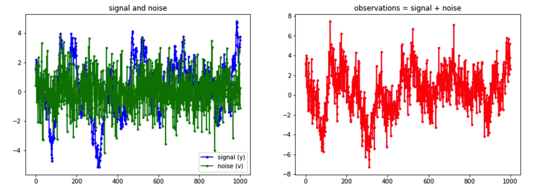

估测经验协方差函数（ESTIMATION OF THE ECF）

# observation mean removal
y0_m = y0 - np.mean(y0)
# max length for ecf evaluation
N2 = int(N/2)
# ecf: xcorr(y0_m, N2)
ecf = np.correlate(y0_m.T[0], y0_m.T[0], mode="full")[len(y0_m)-1-N2:len(y0_m)+N2]

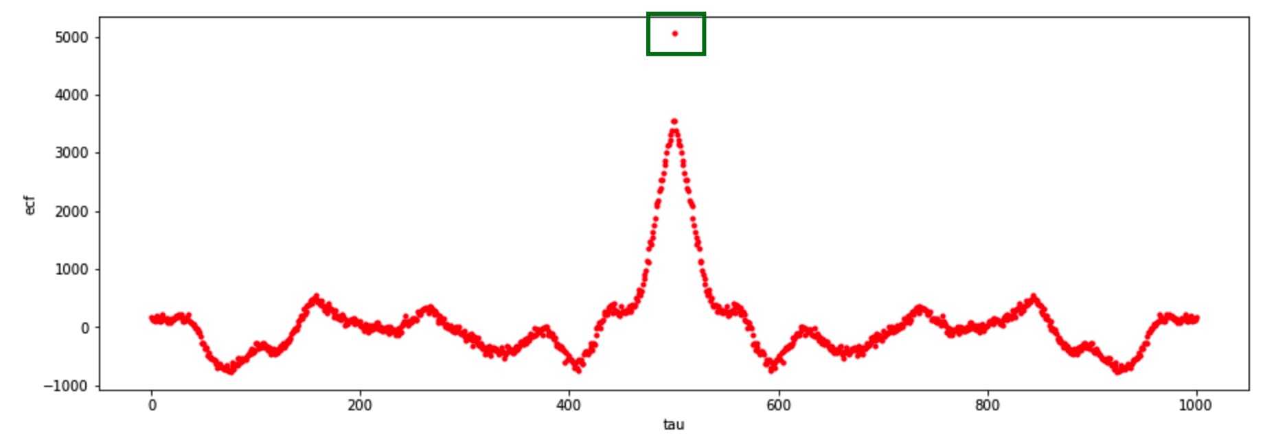
ecf = ecf[N2:2*N2+1].reshape((N2+1, 1))
# biased, definite postive
ecf = ecf / N

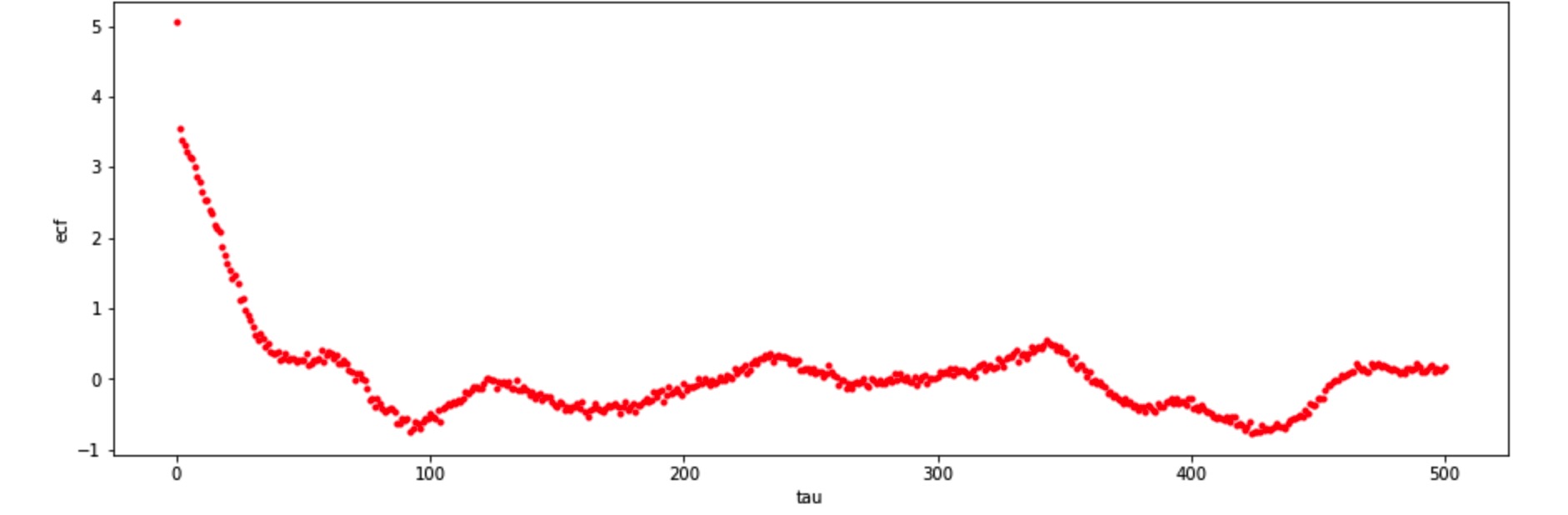
注意：每次运行得到的协方差系数是不一样的，而我们用于计算的模型基于观测值（样本）和噪音。因此，不同的观测值（样本）得到的模型不同。

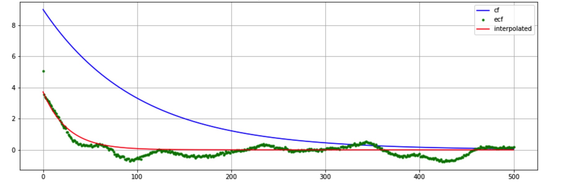
插值法（INTERPOLATION OF THE ECF）估测协方差函数 \(\hat{CF}\)

这里，我们使用指数模型： \[\begin{equation} CF = A_0e^{(-\alpha_0(|t-t'|))} \end{equation}\]

使用最小二乘法（LS）估测参数 \(\hat{A_0}\) 和 \(\hat{\alpha_0}\)。

1. 确定参数的近似值 \(\widetilde{A}\) 和 \(\widetilde{\alpha}\)

利用第 2 和 第 3 个协方差系数来估算 \(\widetilde{A}\)，利用相关长度（correlation length）估算 \(\widetilde{\alpha}\) \[\begin{equation} \begin{aligned} \widetilde{A} &= 2 \times CF(1) - CF(2) \\ \hat{\sigma _{0}}^{2} &= CF(0) - \widetilde{A} \\ \frac{\widetilde{A}}{2} &= \widetilde{A}*e^{(-\widetilde{\alpha}(|\bar{\tau }|))} \\ ln{\frac{1}{2}} &= -\widetilde{\alpha}(|\bar{\tau }|) \\ -ln{2} &= -\widetilde{\alpha}(|\bar{\tau }|) \\ \widetilde{\alpha} &= \frac{ln2}{|\bar{\tau }|} \end{aligned} \end{equation}\]

# approximated values of the parameters for linearization
## intersection with t=0 of the straight line
## exactly interpolating the covariance
## coefficients at step 1 and 2
Ast01 = 2*ecf[1,0] - ecf[2,0]
Ast0 = Ast01
# noise variance estimate
sigma2st0_v = ecf[0,0] - Ast0

ecf_05 = Ast0/2
i_lcorr = np.argwhere(ecf-ecf_05<=0).min(0)[0]
t_lcorr = t[i_lcorr-1,0] # correlation length
# assumption: A/ecf(lcorr) = 2
ast01 = np.log(2)/t_lcorr

# approximated cf model
ecm01 = Ast0 * np.exp(-ast01*t)

2. 迭代估测

这里，我们仅迭代五次：

i_up = np.argwhere(ecf[1:]-ecf[:-1]>=0).min(0)[0]
t_up = t[i_up,0]
#print(i_up, t[1:i_up+1])
# point selection for LS interpolation
t0 = t[1:i_up+1] # confusion here!!!
# ecf values to be interpolated
ecf0 = ecf[1:i_up+1]

# first iteration
Ast = Ast01
ast = ast01

# cf
ecm = Ast * np.exp(-ast*t)
plt.plot(t[:M+1], ecm[:M+1], 'r', label='ecm')
for i in range(5):
    # design matrix (Jacobian)
    A = np.hstack([np.exp(-ast*t0),-Ast*t0*np.exp(-ast*t0)])
    # known terms vector
    a = np.asmatrix(Ast * np.exp(-ast*t0))
    #print(A, A.shape, a.shape, ecf0.shape, t0.shape)
    # estimated parameters
    xst = inv(A.T.dot(A)).dot(A.T).dot(ecf0-a)
    #print(xst, xst.shape)
    # i-th iteration
    Ast += xst[0,0]
    ast += xst[1,0]
    #print(Ast, ast, M)
    # cf
    ecm = Ast * np.exp(-ast*t)
    #print(t.shape, ecm.shape)
    plt.plot(t[:M], ecm[:M], 'r')
    
sigma2st_v = ecf[0,0] - Ast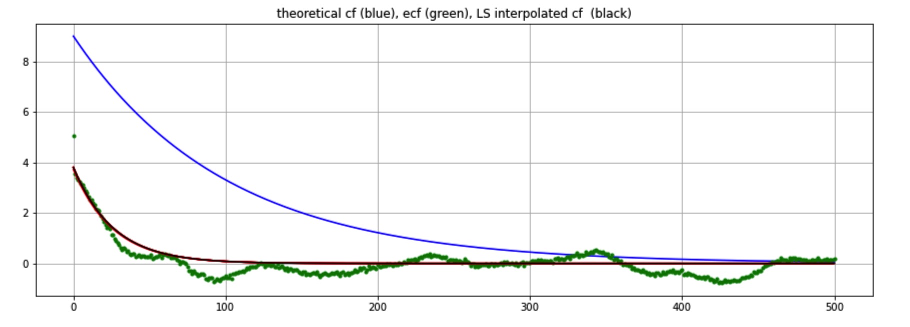

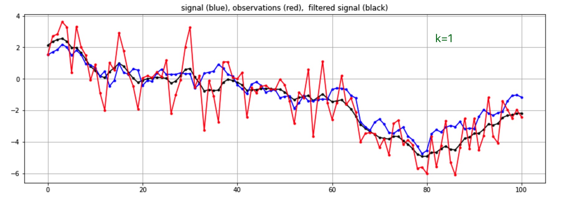
使用观测值和协方差函数 \(\hat{CF}\) 预测指定点集的信号值

• 观测值：\( \underline{y}_0 \)
• 协方差函数： \[\begin{equation} \hat{CF} = \hat{A_0}e^{(-\hat{\alpha_0}(|t-t'|))} \end{equation}\]
• 预测： \[\begin{equation} \hat{y} = C_{yy} \times (C_{yy}+k\times(\hat{\sigma _{0}}^{2}\times I_{N\times N}))^{-1} \times y_0 \end{equation}\]

# number of observations to filter
n = 100

# Covariance matrix of the sampled signal
Cyy = toeplitz(ecm[:n+1])

# Covariance matrix of the sampled signal + noise
Cy0y0 = Cyy + np.eye(n+1)*sigma2st_v

# filtered signal
yst = Cyy.dot(inv(Cy0y0)).dot(y0_m[:n+1])
est = y[:n+1] - yst

print(""" 
estimation error:
   mean\t\t= {}
   std\t\t= {}
""".format(np.mean(est), np.std(est)))

# Covariance matrix of the sampled signal
Cyy = toeplitz(ecm[:n+1])
# Covariance matrix of the sampled signal + noise
Cy0y0 = Cyy + 9*np.eye(n+1)*sigma2st_v

# filtered signal
yst = Cyy.dot(inv(Cy0y0)).dot(y0_m[:n+1])

est = y[:n+1] - yst

print("""
estimation error:
   mean\t\t= {}
   std\t\t= {}
""".format(np.mean(est), np.std(est)))

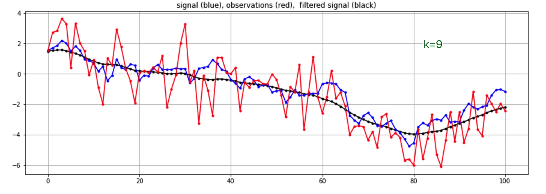
可以看出，k 值越大，noise 的方差越大，估测信号越平滑。

如果我们修改相关长度（correlation length）的大小：

ecmErr = Ast * np.exp(-0.1*ast*t)
Cyy = toeplitz(ecmErr[:n+1])

# Covariance matrix of the sampled signal + noise
Cy0y0 = Cyy + 9*np.eye(n+1)*sigma2st_v # smoother

# filtered signal
yst = Cyy.dot(inv(Cy0y0)).dot(y0_m[:n+1])

est = y[:n+1] - yst

print("""
estimation error:
   mean\t\t= {}
   std\t\t= {}
""".format(np.mean(est), np.std(est)))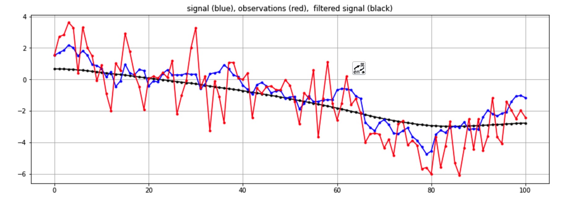

可以看出，相关长度越大，估测信号越平滑；相关长度越小，用以估测信号的观测值越少，估测信号越接近观测值，过滤能力越弱。